Content from R for Music Research
Last updated on 2024-11-19 | Edit this page
Estimated time: 0 minutes
Overview
Questions
- Why should I use R in my music research?
Objectives
- Demonstrate different contexts and use cases showing how R might be used to help answer research questions in music
Introduction
Content from Meet Alex
Last updated on 2024-11-19 | Edit this page
Estimated time: 5 minutes
Say hello to Alex!
Alex is a graduate student studying Music Psychology. Alex is a pianist, and also likes to dabble in music composition. Alex is comfortable using Ableton Live and Logic Pro with MIDI keystations to record and master music.
Alex also spent a summer interning at a Music Label. Responsibilities included entering data in an Excel spreadsheet, producing monthly reports with average duration of listens, most listened to tracks, and most popular artists, and visualising the results using bar graphs. Alex is comfortable carrying out these calculations in Excel, but has no experience doing these calculations using other statistical programmes.
As part of the PhD, Alex is investigating the effect of background music on individuals’ working memory capacity. To do so, Alex ran a study where participants carried out a comprehension task and a working memory task, either in silence, or with background music. The study was run online, and data was collected using a Web-based survey tool. Alex has collected a sufficient number of responses, and now wants to download and analyse the data, to see whether background music had an effect on the participants’ performances in the tasks.
Alex wants to try using R within the RStudio environment to explore and visualise the collected data. Furthermore, Alex wants to document the work carried out, to make it easier to remember what was done when writing up the methodology of the dissertation.
Content from Getting started with R and RStudio
Last updated on 2024-11-19 | Edit this page
Estimated time: 35 minutes
Overview
Questions
- How do I navigate the RStudio user interface?
- How do I run commands in the console?
- What is an R script and how do I create one?
- What are library packages?
- How do I get help?
Objectives
- Navigate the user interface of RStudio
- Run commands in the console and in an R script
- Learn how to install and load a library package
- Look up documentation
The difference between RStudio and R
RStudio is an open-source programme and can be described as an Integrated Development Environment (IDE). One can view RStudio as a tool which helps make working with R more user-friendly. Some of the advantages of using RStudio include an autocompletion function, being able to write code in scripts and save them to be used later on, save objects/variables in the environment, visualise objects, and access to in-depth help documentation on R functions. On the other hand, R on its own comes with a basic interface which is essentially a command-line interface.
During this lesson, we will follow Alex in the exploration of R. We will use RStudio to write out R code, navigate different files on our computer, read data files, inspect objects we create, and visualise plots that we will produce.
Getting around RStudio
When you first open RStudio, you will be presented with the default layout of 3 main panes.
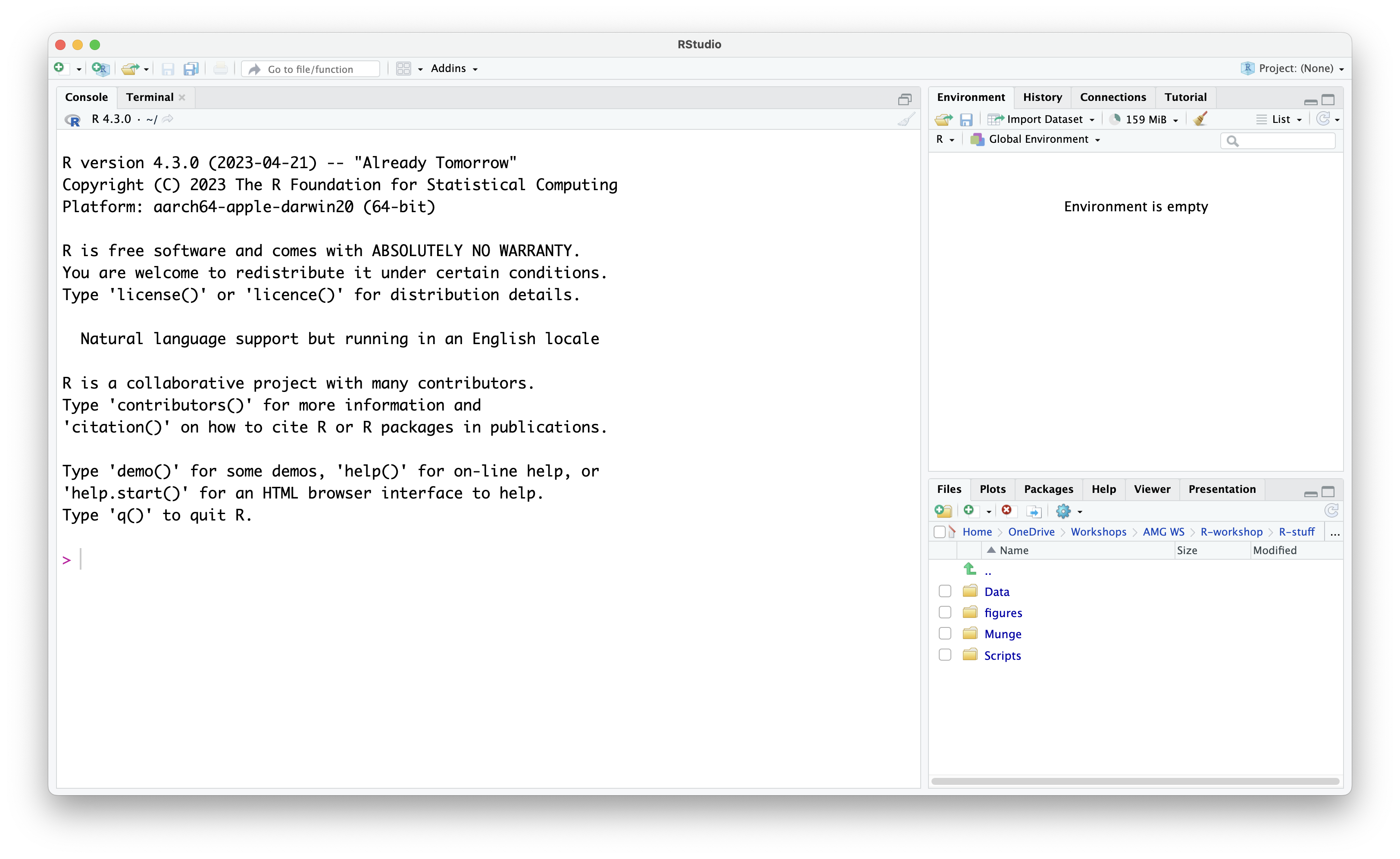
Default Layout:
-
Console Pane (left side of screen): This is the
interface you would use if you were working in R rather than RStudio.
The Console is used to type in and run commands, with the output being
immediately displayed in the Console. A
>symbol and a blinking cursor show you where to input the code. To run commands in the Console, you have to type in the command and press theReturnkey. Code typed directly in the console will not be saved, but you can view it in the History Pane (top right of screen - History tab is the one next to Environment). The Terminal tab next to the Console presents you with a command-line interface which you can use to access your computer’s operating sysem. - Environment Pane (top right of screen): Any data files you read (or “import”) into RStudio will show up here, together with any objects you create in the R environment.
-
Navigation Pane (bottom right of screen): The
Navigation Pane has multiple tabs.
- Files: This tab allows you to view and navigate through the files you have in your current working directory as well as on your computer. New folders and files can be created and existing ones can also be deleted. Other options may be found by clicking on the gear icon.
- Plots: Plots (e.g., bar graphs, scatter plots etc.) created during the R session will be shown in this window.
- Packages: Library packages (explained later in this episode) currently installed are displayed. A ticked box next to a library package represents packages which are loaded in the environment. Library packages can also be installed and/or updated by the respective buttons.
- Help: Any package or function documentation looked up will be displayed in this tab.
- Viewer: The Viewer tab displays web content generated through the session.
- Presentation: Any HTML slides generated during the session will be displayed in this tab.
Note. During this lesson we will not be generating any HTML content, therefore, we will not be using the Viewer and Presentation tabs.
Customise your layout
The placement of these panes can be customised from the Tools > Global Options > Pane Layout menu.
Running commands in the Console vs in an R script
There are two main ways to run commands in RStudio.
Option 1
You can type your commands directly into the Console pane. After typing
in your code, pressing the Return button on your keyboard
will run the command, and R will show the result of your command below
your code in the Console pane. This is a handy way to try out short
lines of code. However, when the code typed in the Console pane will not
be saved and will be lost once you close your RStudio session.
Option 2
You can write your code and save it in a file called an R script, which
will allow you to access your code in subsequent RStudio sessions, by
opening up your R script. This allows you to have a record of all your
code, to be used later by yourself or others.
Creating an R script
To create an R script, select New File > R script from the File menu at the top of the environment. Alternatively, you can click on the icon showing a white square overlaid by a white cross in a green circle and select R script from there. This action will create an empty R script, which will appear in the top left pane. This is now the R script editor, where you can type your code in the R script file. The RStudio layout has now changed to display 4 panes instead of the original 3.

R scripts have .R as their file extension. Since typing
up commands in an R script is similar to typing words in a text editor,
pressing the Return key will not run your commands (like
what happens in the Console pane), but it will create a new line for you
to write more code. To run the code that you type in an R script, you
have to tell RStudio to push your code from the R script to the Console.
Once pushed to the Console, the code will be executed, and the results
of the code will appear in the Console.
To run a line of code in your R script, make sure that your cursor is
on the line of the script that you want to run, and then press the
Run button at the top of the Editor pane.
Shortcut to run R script code
Instead of pressing the Run button at the top of the
Editor pane, you can either:
- Press
Ctrl+Returnon Windows or Linux, orCommand+Returnon Mac - Select the line or lines of code you want to run, and from the Code menu, select Run selected line(s)
Don’t forget to save your work
Make sure to save your R script by either pressing the floppy disk (a small light blue and white square) icon on the Editor pane, or by selecting Save from the File menu at the top. On your first save, you will be prompted to give your R script a name and select the location where you want to save your file.
The shortcut Ctrl + s on Windows and Linux,
or Command + s can also be used to save your
file.
Library packages
Default R comes with what are called base functions. However, R users have also created other packages which hold different tools that can be added to R, to help extend R’s capability, depending on what you want to use it for. Packages can be downloaded from the Comprehensive R Archive Network known as CRAN.
One package that we will be using is the dplyr package,
which allows us to subset and manipulate parts of a dataset, to have a
closer look at certain elements - so let’s download it. To do so, we
first need to install it and then load it into our R environment by
following these two steps:
Step 1 - Install the package
R
install.packages('dplyr')
OUTPUT
The following package(s) will be installed:
- dplyr [1.1.4]
These packages will be installed into "~/work/intro-to-R-for-MRs/intro-to-R-for-MRs/renv/profiles/lesson-requirements/renv/library/linux-ubuntu-jammy/R-4.4/x86_64-pc-linux-gnu".

# Installing packages --------------------------------------------------------
- Installing dplyr ...                          OK [linked from cache]
Successfully installed 1 package in 6.1 milliseconds.
Step 2 - Load package
R
library(dplyr)
OUTPUT
Attaching package: 'dplyr'OUTPUT
The following objects are masked from 'package:stats':

    filter, lag
OUTPUT
The following objects are masked from 'package:base':

    intersect, setdiff, setequal, union
Exercise: Install and load packages
Further on, Alex will want to create plots for some data. For this,
we need to install and load the ggplot2 package. Complete
the following code to first install the ggplot2 package and
then load the package in your R environment.
Step 1 - Install package
install.______('_____')Step 2 - Load package
library(_____)Step 1 - Install package
R
install.packages('ggplot2')
OUTPUT
The following package(s) will be installed:
- ggplot2 [3.5.1]
These packages will be installed into "~/work/intro-to-R-for-MRs/intro-to-R-for-MRs/renv/profiles/lesson-requirements/renv/library/linux-ubuntu-jammy/R-4.4/x86_64-pc-linux-gnu".

# Installing packages --------------------------------------------------------
- Installing ggplot2 ...                        OK [linked from cache]
Successfully installed 1 package in 6.1 milliseconds.
Step 2 - Load package
R
library(ggplot2)
Let’s have a look at our loaded packages. To view all packages loaded in our R environment, run the following command:
R
(.packages())
OUTPUT
[1] "ggplot2"   "dplyr"     "stats"     "graphics"  "grDevices" "utils"
[7] "datasets"  "methods"   "base"
Getting help in R
R provides access to in-built documentation on any R function. To
access this information, you can use the help() function,
where you input the name of the function within the brackets of the
aforementioned function. For example, if you want to look up the
documentation on the mean function, which calculates the
average of a calculation, you enter help(mean) in the
terminal and press Return.
R
help("mean")
The R documentation, which includes a brief description of the
function, the arguments that can be inputted in the mean
function, as well as some examples of how the function is used, will
show up in the Help pane on the right-hand side of the RStudio
environment. As a shortcut to the help() function, you can
use the ? help operator to look up the same documentation
in this way:
R
?mean
Exercise: Getting help
Alex wants to look up the mean command, but instead of
using help(), Alex used help.search().
However, this command outputted different search results.
- Run
help("mean")in the console, and look at the results in the Help pane - Do the same with the
help.search("mean")command - What is the difference?
Running the two commands consecutively:
R
help("mean")
R
help.search("mean")
The help("mean") command gave Alex the relevant help
page for the mean function. On the other hand, the
help.search("mean") function gave Alex a list of links to
help pages, vignettes, and code demonstrations where the keyword
mean was present.
The help("mean") command works well if you know the
exact name of the function you want to look up. However, sometimes, one
may be unsure of the exact name of a function. This is where the
help.search() function comes in handy. This function will
search through all R documentation, as well as installed packages and
online resources for functions and packages which contain the keyword
inputted, and will display the results in the Help pane as links to all
functions and packages containing the keyword.
A shortcut
Instead of help.search(), you can also use its
equivalent shortcut ??
R
??mean
Getting help outside of R
There are numerous resources that offer helpful information on R. A non-exhaustive list includes:
- Stack Overflow
- CRAN
- R for Data Science by Wickham, Çetinkaya-Rundel, and Grolemund
- Cheatsheets of different R packages provided by posit (the website also contains cheatsheets of other programming languages e.g., Python)
- Other The Carpentries lessons on R
Testing out instructor notes
Key Points
- Write your code in an R script to be able to save it
- Run code in an R script using
Command+Returnon Mac,Ctrl+Returnon Windows/Linux, or by pressing the Run button - Use
install.packages()to download and install a library package - Use
library()to load the downloaded package in your environment - Use
help(),help.search()and the?and??help operators to look up documentation on commands and packages
Content from Creating a directory structure
Last updated on 2024-11-19 | Edit this page
Estimated time: 0 minutes
Overview
Questions
- What is a working directory?
- How do I set up a new working directory?
- How do I create new directories?
- How do I check what files are in my directory?
Objectives
- Set up a working directory
- Confirm the current working directory
- Create a directory structure
- Navigate through your directory
The working directory
Before starting working on the project, Alex wants to make sure that work is done in an organised way by using a consistent folder structure. This will make it easy to find things in the future.
First, Alex needs to set up a working directory.
What is a working directory?
The word directory may be viewed as another word for folder. Since one might have a lot of files and folders on their device, we need to let R know which directory (folder) we will be working in, so that R knows where to look for files to use, open, and also save. We can set up our working directory through RStudio.
Let’s first check what our current working directory is.
To do so, we will use the getwd() function (which stands
for get working directory).
R
getwd()
Reminder: Use of R script vs Console
You can type the commands directly in the Console, and press
Return to execute the command. Remember that commands typed
directly in the Console will not be saved. Since it might be useful to
have a saved copy of the code used throughout this R lesson, it is
recommended that you use an R script instead. Remember that to execute
line(s) of code in an R script, you have to put your cursor on the
desired line (or select multiple lines) that you want to run, and press
Command + Return on Mac or Ctrl +
Return on Windows and Linux.
The output to getwd() will be different for everyone,
but it may look something like:
"/Users/yourusernamehere"
For example, Alex’s working directory is:
"/Users/alex"
Alex wants to set the working directory to an existing folder called
my-r-project.
To do so, Alex needs to tell R to change the working directory to
my-r-project by using the setwd() function and
typing in the pathname of the folder.
R
setwd("/Users/alex/Desktop/my-r-project")
When this command is run, no output will be shown in the Console. We
can use the getwd() command to check whether R has set the
desired folder as the working directory.
R
getwd()
Alex has now confirmed that R is seeing the my-r-project
as the working directory.
Good to know
You can also set your working directory by navigating through your device’s system in the Files pane (bottom right pane), going into the folder you want as your working directory, clicking on the cogwheel icon and selecting Set as working directory.
Organise the working directory
Now that Alex has set up the desired working directory, Alex wants to
organise the files to be used in this project in the following folder
structure within the working directory (my-r-project):
- data/ Alex will put the raw data files (and other data) in this folder
- figures/ Any plots and graphics created will be saved in this folder
- scripts/ All R scripts written by Alex will be saved here
- munge/ This folder will hold all data cleaning and data manipulation R scripts
- documents/ Alex will use this folder for the research report and any written drafts
Good to know
There is no specific folder structure that needs following - the folder structure is completely up to you, however, having some sort of folder structure to organise your files is recommended.
There are multiple ways that folders (or directories) may be created in RStudio.
Alex will use the dir.create() function to create the
desired folder (directory).
R
dir.create("data")
Alex has now created the first folder within the working directory.
However, Alex is not sure whether this was done correctly, as this
command did not output a result in the Console. To confirm that the
data folder was created, Alex used the
list.files() function, which will display all items in the
working directory.
R
list.files()
Exercise: Directory structure
- Create the following folders in the working directory:
figures,scripts,munge, anddocuments - Check that all folders are now in your working directory
Alternatively, new folders can be created through the Files pane (bottom right pane in environment) by clicking on the new folder icon.

Folders can also be created outside of RStudio through File Explorer/Manager on Windows and Linux, and Finder on Mac.
Key Points
- The term ‘directory’ in R has the same meaning as the common term ‘folder’
- Use
getwd()to check your current working directory - Establish a new working directory with
setwd() - Create new directories using
dir.create("nameofnewdirectoryhere")or through the navigation pane - Use
list.files()to view all files in your working directory
Content from Reading survey data in R
Last updated on 2024-11-19 | Edit this page
Estimated time: 0 minutes
Overview
Questions
- How do I import csv and Excel data files in R?
- How can R deal with missing values on import?
- How do I give names to the data set imported?
Objectives
- Import Excel and csv files in R
- Specify how to deal with missing values
- Create an object for your imported data
Introducing our dummy data set
During this and the following episodes, we will be using a dummy data set as an example of survey data. The dummy data set is inspired by a study about the effect of background music on individuals’ working memory capacity carried out by Lehmann and Suefert, 2017. Our fake study consisted of participants carrying out a comprehension task and a working memory task in one of the two conditions: in silence, or with background music. Participants also rated their mood and arousal on 5-point scales, and demographic information such as musicianship and age was collected. The fake study was run online, and data was collected using a Web-based survey tool. We will use R to explore the data set, and analyse the data, to see whether background music had an effect on our fake participants’ performances in the tasks.
But first, we need to download the files and import the data into R.
Download the data files here.
Reminder: Files need to be in the working directory
Remember that R needs to know in which directory to look for files to be used and/or saved. The data files downloaded should be put in the directory set up in Episode 4.
- To check what your working directory is set to, use
getwd().
- To set a new working directory, use
setwd("pathway here"), or go into the desired folder through the Files Pane and click on the Cogwheel and select Set as working directory.
Dummy data set formats
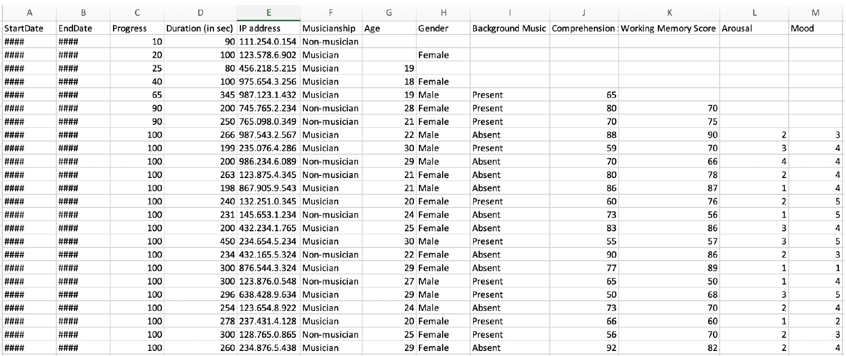
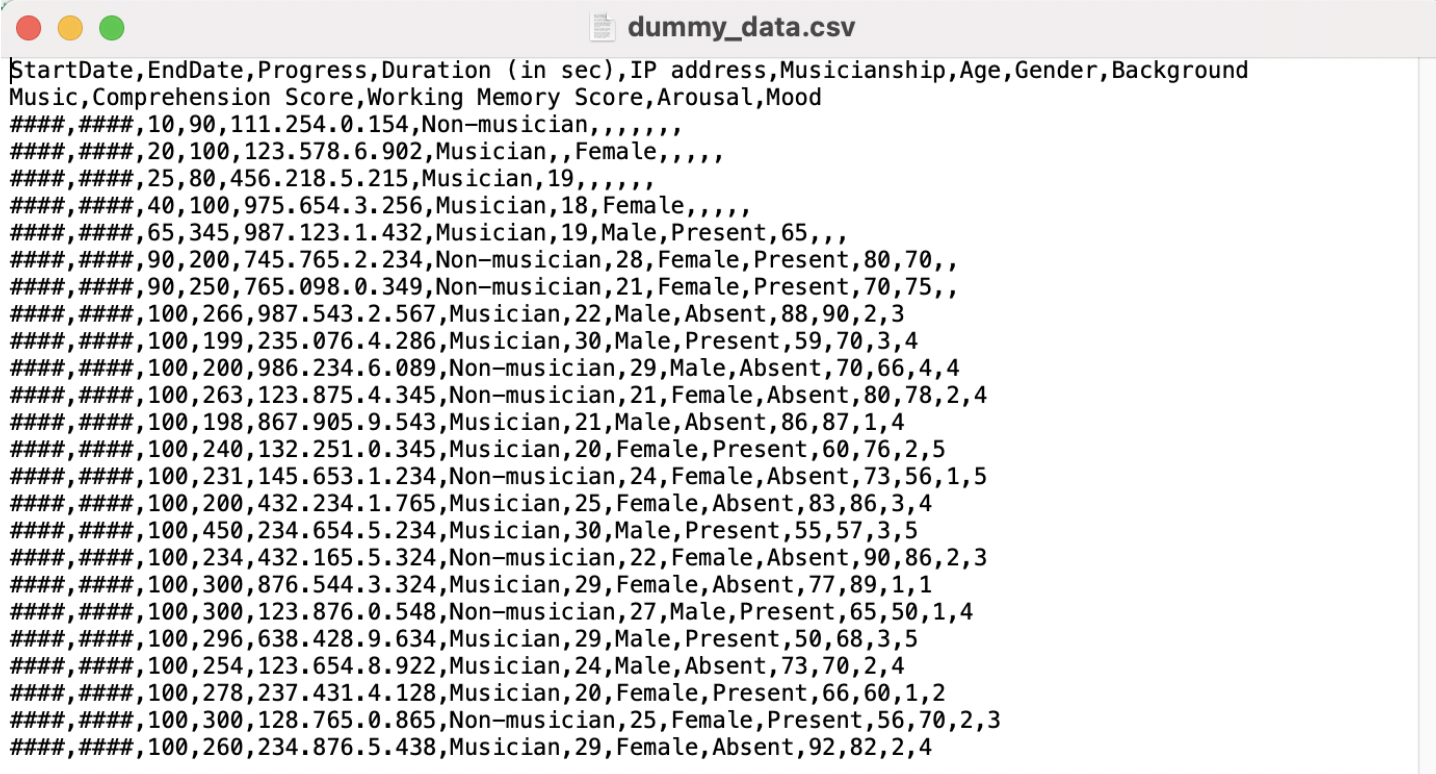
Our dummy data set files come in two formats: an Excel file and a csv file.
When opening our dummy_data.xlxs file in Excel, we are presented with the data in this manner:
When opening our dummy_data.csv file using a text editor, our data looks something like this:
To test out how R handles both types of data files, we will first import the Excel file, and then the csv file in R.
Importing an Excel data file
An Excel file can be imported in R using the library package
readxl. We need to install and load the library package by
following the steps used in Episode
3 of this lesson, before we can use it.
Exercise: The readxl package
Install and load the readxl package
Step 1: Install the package
R
install.packages("readxl")
OUTPUT
The following package(s) will be installed:
- readxl [1.4.3]
These packages will be installed into "~/work/intro-to-R-for-MRs/intro-to-R-for-MRs/renv/profiles/lesson-requirements/renv/library/linux-ubuntu-jammy/R-4.4/x86_64-pc-linux-gnu".

# Installing packages --------------------------------------------------------
- Installing readxl ...                         OK [linked from cache]
Successfully installed 1 package in 6.2 milliseconds.
Step 2: Load the library package in your R environment
R
library(readxl)
TIP
A quick way to check whether a library package was loaded in your environment or not, is to go to the Packages pane (bottom-right) and the Search function, look up the name of your library package. A tick should be displayed next to the library package name, indicating that the package is loaded.
We will now load our Excel data file into R, and assign our data file a name so that we can store it in our RStudio environment - in other words, saving our file in R’s memory. To do so, we will use the assign operator which is <-.
We will call our data file exceldata.
R
exceldata <- read_excel("dummy_data.xslx")
Once this command is run, an object with the name
exceldata showing the number of observations and variables
should be present in the Environment pane (top right).
Let us now import our csv file into R.
Importing a csv data file
We will use the read.csv() function to import our csv
file. Similarly, we will give our csv data file a name and ‘save’ it in
our R environment. We will call this data file csvdata.
R
csvdata <- read.csv("dummy_data.csv")
This new object or variable can now be seen in our Environment pane.
A good place for a checkpoint, to make sure everyone is up to speed. Approx. time ~ 11 min up to here.
Exercise: Representation of our two data files
Let’s look at the contents of our exceldata in R using
View(exceldata). The contents of exceldata
should open up in a new tab. Use the same function to view the contents
of csvdata.
Compare how the data files were represented in Excel and a text
editor (images above) to how exceldata and
csvdata are represented in R. Do you notice any differences
or similarities?
Write down your answers in the Etherpad.
Data in Excel is presented in tabular format (the rows and columns) in cells. When we opened the .csv file outside of R, our data was not presented in a tabular format, but as a text file with data separated by commas (hence comma seperated values). However, R stored both data file formats as tabular data.
Excel vs csv
Although we could work with both Excel or csv files, in this lesson we will continue working with our data in csv format.
csv files tend to be favoured as a data file format for a couple of reasons:
- csv is in plain text format and can be read with any text editor
- text editors cannot edit files saved in Excel format
- csv files do not need any specific platform to open, whilst Excel files need specific applications
- csv files consume less memory than Excel files
- csv fils are generally faster than an Excel file
Since we do not need the exceldata anymore, we will
remove this from our R environment (i.e., we will remove this from R’s
memory) using rm(exceldata).
Dealing with missing values
More often than not, our data will contain some missing values, perhaps because certain participants did not complete the survey, or maybe there were some optional questions which participants opted to skip.
One way to deal with missing values is at the data import stage. Most
funtions in R tend to have several arguments (or settings) that
you can specify. One of the arguments of the read.csv()
function that comes in handy in these cases is the
na.strings.
The na.strings argument allows you to specify which
values in your data set should be interpreted as NA values.
For example, for blank fields to be considered as missing values when importing a data file, we could write the following code:
R
ourdata <- read.csv("dummy_data.csv", na.strings = NA)
We can also specify any words (i.e., data of character type) that should be regarded as missing values, such as the words “NA” written down in a field:
R
ourdata <- read.csv("dummy_data.csv", na.strings = "NA")
Note. Here we put NA in “” since in this case NA is written text.
Exercise: NAs in our data
Have a look at our csvdata and try to spot missing
values in the data. Make a note of all representations of the missing
data (e.g., blank fields, text such as “n/a” being used, etc.).
Let’s import our csv file once again in R, but this time adding the
na.strings argument in the read.csv()
function, specifying all values in the data that should be regarded as
missing values.
HINT: To combine multiple items in the
na.strings argument, use the following syntax:
na.strings = c("A", "B, "C")
View this new object. What can you observe?
In our data we have blank fields but also the use of the text “N/A” and “n/a” which should be regarded as missing values.
To import our data file excluding all of the above, we write the following code:
R
ourdata <- read.csv("dummy_data.csv", na.strings = c(NA, "N/A", "n/a"))
When we view ourdata, we can now see that any instances
of written text with “N/A” and “n/a” are also being regarded as missing
values.
GOOD TO KNOW
The read_excel() function has a similar argument called
na:
R
exceldata <- read_excel("dummy_data.xlsx", na = "N/A")
Now that we have our data file with the na.strings
argument, we can remove the first csvdata created, and move
on to inspecting our data in the next episode.
Key Points
- Use
read.csv()to import a csv data file in R - Use
read_excel()from thereadxlpackage to import an Excel data file in R - Use the assign operator
<-to give a name to your data set - Specify how to deal with missing values using the
na.stringsargument inread.csv()when importing a csv file
Content from Inspecting your data in R
Last updated on 2024-11-19 | Edit this page
Estimated time: 0 minutes
Overview
Questions
- How many rows and columns are in my data frame?
- What are the names of the columns in my data frame?
- How can I look up parts of my data frame?
- How do I find out what the internal structure of my data frame is?
Objectives
- Determine the number of rows and columns in a data frame
- Look up the names of the columns in a data frame
- Pull up sections of a data frame
- Inspect the internal structure of a data frame
Key Points
- Inspect the dimensions of a data frame using
dim() - Find out the number of rows and columns of a data frame using
nrowandrcol - Use
colnames()andrownames()to display column and row names respectively - Use
head()to view the first six rows of a data frame - Look at data in a specific column by using the
$operator - Use
[]to subset data from a data frame - Use
str()to inspect the internal structure of the data frame
Content from Cleaning your data
Last updated on 2024-11-19 | Edit this page
Estimated time: 0 minutes
Overview
Questions
- What are some steps I should take to clean my data before use?
- How do I identify and deal with missing values in the data?
- How do I save my cleaned data into a new data file?
Objectives
- Eliminate irrelevant data
- Remove data with a low completion rate
- Rename data columns which have lengthy or confusing names
- Identify missing values in the data
- Add a Participant ID column
- Save the cleaned data as a new data file
Key Points
- Use the
select()function from thedplyrpackage to remove unneccesary data columns - Use the
filter()function to omit data based on a specific parameter - Use
is.na()to identify missing values in the data - Use
na.omit()to exclude rows with any missing data - Use
write.csv()to save the cleaned data as a new data file
Content from Analysing survey data
Last updated on 2024-11-19 | Edit this page
Estimated time: 0 minutes
Overview
Questions
- What are some descriptive statistics of my data set that I can compute in R?
- How do I calculate the number of participants in my survey data?
- How do I calculate the mean age of participants in my survey data?
- How do I found out what age are the youngest and oldest participants in my survey data?
- How do I compare scores of participants based on their musicianship?
- How do I carry out a t-test?
Objectives
- Calculate the number of participants in your survey data
- Calculate the mean age and standard deviation of participants
- Determine the number of musicians and non-musicians that took part in your survey
- Calculate the average scores of musicians and non-musicians separately
- Carry out a t-test to find out if musicianship had a statistically significant effect on how participants scored on their tasks they had to carry out
Key Points
- Use
mean()andsd()to calculate the mean and standard deviation of a variable - Use
min()to identify the minimum value of a particular variable - Use
max()to identify the maximum value of a particular variable - Include the
na.rm = TRUEargument in functions when possible for the calculation to ignore missing values in the data - Use
filter()to subset your data by a specific variable - Use the
t.testfunction with the following syntaxt.test(DependentVariable ~ IndependentVariable, data)to compare whether the means of two groups are statistically different or not
Content from Visualising survey data with ggplot2
Last updated on 2024-11-19 | Edit this page
Estimated time: 0 minutes
Overview
Questions
- What are the 3 main components of a ggplot?
- How do I create a scatterplot, boxplot, and a bar graph to visualise my data?
- How can I create separate plots at once based on a variable of my data?
- How do I customise my plots to add axes labels and a title?
- How do I save my plots in png format?
Objectives
- Gain an understanding of how to create a plot using the
ggplot2package - Create a scatterplot, boxplot, and bar graph
- Create separate plots at once based on a variable in the data
- Give your plot a title and axes labels
- Save your plot
Key Points
- A ggplot has 3 main components: data, aesthetics, and geom
- A ggplot may be customised by adding layers of elements
- Use
geom_point()to create a scatterplot,geom_boxplot()for a boxplot, andgeom_bar()for bar graphs - Use
facet_wrap(~variable)to create separate plots simultaneously based on the unique values of a variable - Give your plot a title with
ggplot('title here')and label your axes withylab()andxlab() - Save your plot with
ggsave()
Content from A second case study for music research
Last updated on 2024-11-19 | Edit this page
Estimated time: 0 minutes
Overview
Questions
- Can I apply what I learnt about R for a different case study?
- How do I read data from an online dataset in R?
- How can I look up specific parts of the dataset?
- How can I visualise specific parts of the dataset?
Objectives
- Explore a larger dataset using the same methods introduced in the previous episodes
- Recognise that you can use the same code to explore different datasets, irrelevant of their size
Key Points
- An advantage of using R to work with data is that the same code can be run for different data sets of different sizes, subject to the data sets being in similar formats
Content from Some best practices when writing code in R
Last updated on 2024-11-19 | Edit this page
Estimated time: 0 minutes
Overview
Questions
- What are some best practices to keep in mind when writing code in R?
Objectives
- Strive to keep files organised in a structured directory
- Be aware of any dependencies for your code
- Produce code which can be reproducible by yourself and others by documenting your code with comments
Key Points
- Keep your files organised in your working directory
- Consider your working directory and what is required to reproduce your code (e.g., packages)
- Be consistent in your naming conventions
- Use
#to add comments to your code